1 Data

The data I used for analysis is called - Default.

The Default data set resides in the ISLR package of the R programming language. It contains selected variables and data for 10,000 credit card users.Some of the variables present in the default data set are:

• student - A binary factor containing whether or not a given credit card holder is a student.

• income - The gross annual income for a given credit card holder.

• balance - The total credit card balance for a given credit card holder.

• default - A binary factor containing whether or not a given user has defaulted on his/her credit card.

The goal of this investigation is to fit a model such that the relevant predictors of credit card default are elucidated given these variables. You can find the data structure from below section.

head(Default)

##   default student   balance    income
## 1      No      No  729.5265 44361.625
## 2      No     Yes  817.1804 12106.135
## 3      No      No 1073.5492 31767.139
## 4      No      No  529.2506 35704.494
## 5      No      No  785.6559 38463.496
## 6      No     Yes  919.5885  7491.559

str(Default)

## 'data.frame':    10000 obs. of  4 variables:
##  $ default: Factor w/ 2 levels "No","Yes": 1 1 1 1 1 1 1 1 1 1 ...
##  $ student: Factor w/ 2 levels "No","Yes": 1 2 1 1 1 2 1 2 1 1 ...
##  $ balance: num  730 817 1074 529 786 ...
##  $ income : num  44362 12106 31767 35704 38463 ...

2 Income, Balance & Default

What variables we are going to use for this analysis? So, in the Defaultdata, the key variables are income, balance, and credit card default (default).

The Key question is-"Is there a relationship between income, balance, and student status such that one, two, or all of these might be used to predict credit card default?"

First, the necessary packages and data are loaded to R, for the illustration purpose. (I’ve already loaded all the necessary packages at the beginning of the file).

library(ISLR)
library(dplyr)
library(ggvis)
library(boot)

Then, a Scatterplot and a box-plot are plotted to investigate the potential relationship between variables.

From the scatter plot shown below, it seem to suggest that there is a relationship between credit card balance and default, while income is not related. This relationship is further confirmed by the boxplot figure below between credit card baland and default.

# Basic scatter plot
ggplot(Default, aes(x=balance, y=income, shape=default, color=default)) + geom_point()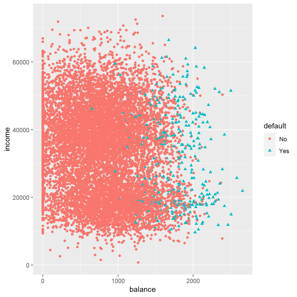

ggplot(Default) + aes(x = default, y = balance, color=default) +
  geom_boxplot(outlier.colour="red", outlier.shape=2,
                outlier.size=1)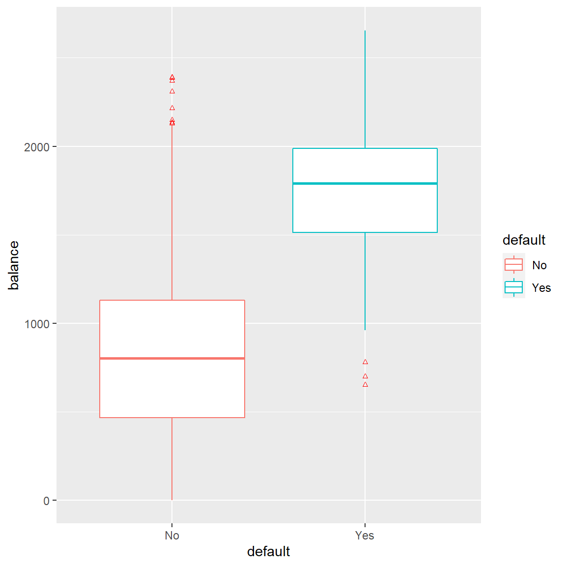 

3 Model Selection

Based on above plots, it suggests that credit card balance, but not income, is a useful predictor of default status. However, to be thorough in the investigation we will begin by fitting all parameters to a model of logistic form.

The logistic regression model is selected to fit in the credit card data because it is:

1. highly interpretable
2. the model does well when the number of parameters is low compared to N observations
3. relatively quick operating time in R and
4. fits the binary (default/non default) nature of the problem well.

This model yields the following coefficients and model information.

glm(default~balance + student + income, family = "binomial", data = Default)

## 
## Call:  glm(formula = default ~ balance + student + income, family = "binomial", 
##     data = Default)
## 
## Coefficients:
## (Intercept)      balance   studentYes       income  
##  -1.087e+01    5.737e-03   -6.468e-01    3.033e-06  
## 
## Degrees of Freedom: 9999 Total (i.e. Null);  9996 Residual
## Null Deviance:       2921 
## Residual Deviance: 1572  AIC: 1580

4 Diagnosis

An ANOVA test using Chi-Squared and the summary statistic p-values suggests that both balance and student status are useful for predicting default rates. (i.e both the Chi-Squared and p-values are statistically significant.)

my_logit <- glm(default~balance + student + income, family = "binomial", data = Default)
anova(my_logit, test = "Chisq")

## Analysis of Deviance Table
## 
## Model: binomial, link: logit
## 
## Response: default
## 
## Terms added sequentially (first to last)
## 
## 
##         Df Deviance Resid. Df Resid. Dev  Pr(>Chi)    
## NULL                     9999     2920.7              
## balance  1  1324.20      9998     1596.5 < 2.2e-16 ***
## student  1    24.77      9997     1571.7 6.459e-07 ***
## income   1     0.14      9996     1571.5    0.7115    
## ---
## Signif. codes:  0 '***' 0.001 '**' 0.01 '*' 0.05 '.' 0.1 ' ' 1

summary(my_logit)

## 
## Call:
## glm(formula = default ~ balance + student + income, family = "binomial", 
##     data = Default)
## 
## Deviance Residuals: 
##     Min       1Q   Median       3Q      Max  
## -2.4691  -0.1418  -0.0557  -0.0203   3.7383  
## 
## Coefficients:
##               Estimate Std. Error z value Pr(>|z|)    
## (Intercept) -1.087e+01  4.923e-01 -22.080  < 2e-16 ***
## balance      5.737e-03  2.319e-04  24.738  < 2e-16 ***
## studentYes  -6.468e-01  2.363e-01  -2.738  0.00619 ** 
## income       3.033e-06  8.203e-06   0.370  0.71152    
## ---
## Signif. codes:  0 '***' 0.001 '**' 0.01 '*' 0.05 '.' 0.1 ' ' 1
## 
## (Dispersion parameter for binomial family taken to be 1)
## 
##     Null deviance: 2920.6  on 9999  degrees of freedom
## Residual deviance: 1571.5  on 9996  degrees of freedom
## AIC: 1579.5
## 
## Number of Fisher Scoring iterations: 8

5 Interesting Points

In the process of modeling, an interesting point presented itself:

When fitting the student status parameter against default, the coefficent for our model is a positive value, implying that student status increases default. When fitting all parameters in our model, the value becomes negative, implying that student status reduces the probability of default.

How can this be?

# single x model
my_logit2 <- glm(default~student, family= "binomial", data = Default)
summary(my_logit2)$coef

##               Estimate Std. Error    z value     Pr(>|z|)
## (Intercept) -3.5041278 0.07071301 -49.554219 0.0000000000
## studentYes   0.4048871 0.11501883   3.520181 0.0004312529

# complex model
summary(my_logit)$coef

##                  Estimate   Std. Error    z value      Pr(>|z|)
## (Intercept) -1.086905e+01 4.922555e-01 -22.080088 4.911280e-108
## balance      5.736505e-03 2.318945e-04  24.737563 4.219578e-135
## studentYes  -6.467758e-01 2.362525e-01  -2.737646  6.188063e-03
## income       3.033450e-06 8.202615e-06   0.369815  7.115203e-01

Looking at the plot below, the data suggests that balance and student status are correlated. Therefore, it might be appropriate to offer the following interpretation: students tend to have higher balances than non-students, so even though a given student has a lesser probability of default than a non student, (for a fixed balance) because students tend to carry higher balances overall, students tend to have higher, overall default rates.

ggplot(Default) + aes(x = student, y = balance, color=student) +
  geom_boxplot(outlier.colour="red", outlier.shape=2,
                outlier.size=1)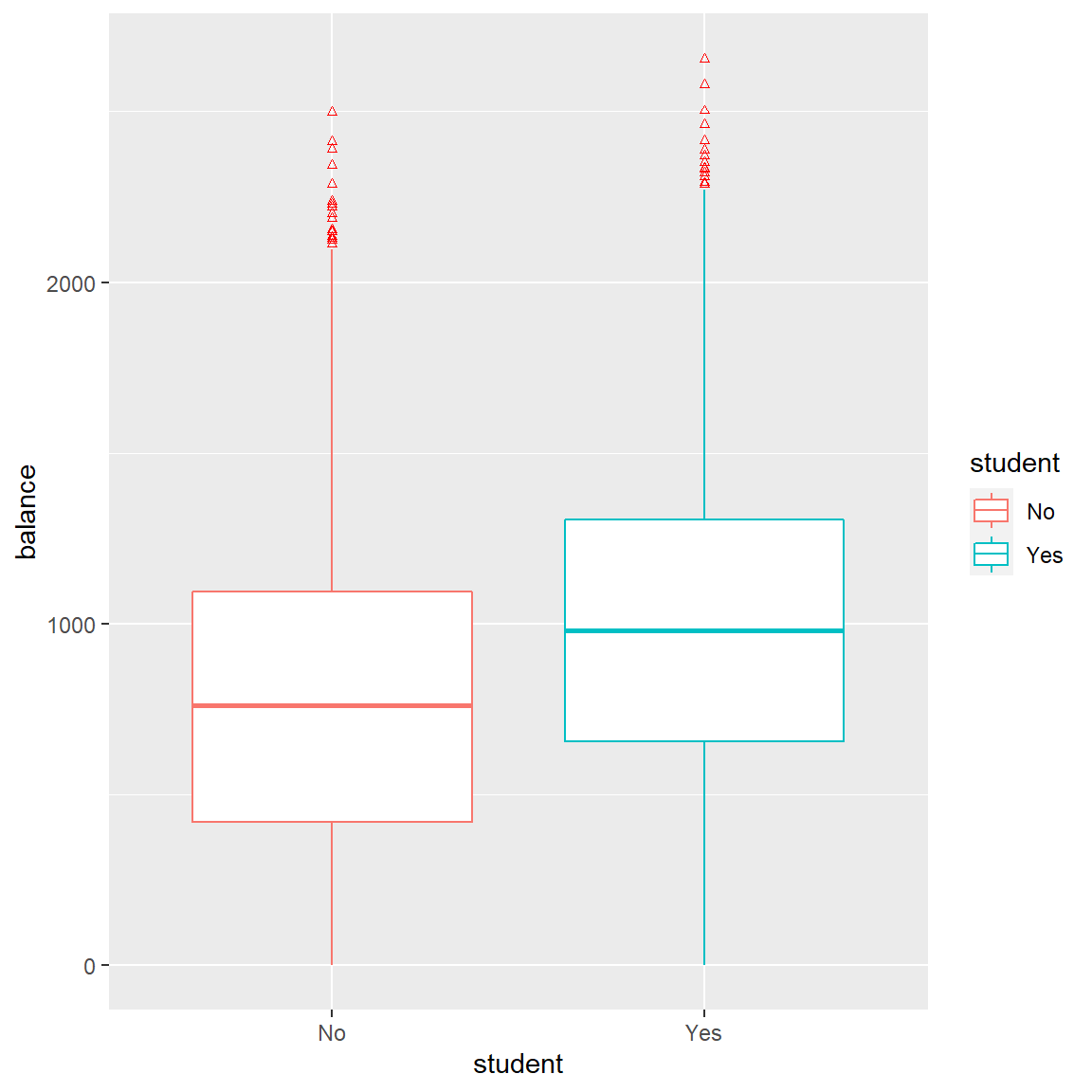 

6 Model Cross-Validation

Just as important as it is to choose a model that fits the parameters correctly, it is even more so to test the predictive power of the chosen model. To do so, I chose to perform:

1. validation set verification and
2. K-fold cross-validation set with 3, 5, and 10 folds.

The results of the validation set are below:

set.seed(1)

# Create a sample of 5000 observations
train <- sample(10000,5000)

A new dataset is generated-Defaultx. DeFaultx is a subset of the Default data that does not include the training data that we will fit the model on. Then, we fit the logistic model to this .

# Generate Defaultx (test data)
Defaultx <- Default[-train,]


# Fit the logistic model using the training data.  
# Be aware of the subset option (subset=train).
glm.fit <- glm(default~ balance + student, data = Default, family = binomial, subset = train)

(glm.fit) # Check the degrees of Freedom (4997)

## 
## Call:  glm(formula = default ~ balance + student, family = binomial, 
##     data = Default, subset = train)
## 
## Coefficients:
## (Intercept)      balance   studentYes  
##  -10.660025     0.005769    -0.979274  
## 
## Degrees of Freedom: 4999 Total (i.e. Null);  4997 Residual
## Null Deviance:       1524 
## Residual Deviance: 802.3     AIC: 808.3

# Use the logistic model to fit the same logistic model, but use the test data.  
glm.probs <- predict(glm.fit, Defaultx, type = "response")

# Make a vector that contains 5000 no responses.   
glm.pred <- rep("No", 5000)

# Replace the "no reponses" in the glm.pred vector where the probability is greater than 50% with "Yes"
glm.pred[glm.probs > .5] = "Yes"

# Create a vector that contains the defaults from the testing data set, Defaultx
defaultVector <- Defaultx$default 

# Calculate the mean of the values where the predicted value from the training equals the held out set.  
mean_df <- mean(glm.pred == defaultVector)

pct_df <- paste(100*mean_df,"%",sep="")

Using the technique above, we can see that 97.4% of the observations in the test set were classified correctly using the logistic model training set. As this is just one of a variety of validation methods, for technical completeness, below we also implement a K-Fold cross validation set:

# Seed the random number generator 
set.seed(2)

# Fit a logistic model using default and income values
glm.fit1 <- glm(default~balance + student, data = Default, family = binomial)

# Create a vector with three blank values
cv.error <- rep(0,3)

# Store the results of each K  validation set into cv.error.  Use K= {3,5,10} 
cv.error[1] <- cv.glm(Default, glm.fit1, K=3)$delta[1]
cv.error[2] <- cv.glm(Default, glm.fit1, K=5)$delta[1]
cv.error[3] <- cv.glm(Default, glm.fit1, K=10)$delta[1]

mean_df2 <- 1 - mean(cv.error)

pct_df2 <- paste(100*round(mean_df2,digits=4),"%",sep="")

We interpret the value of (1-mean(error)) to be the average of the correctly validated observations of the data set using the K-Folds technique. The results of this are also promising! We can see that again approximately 97.86% of values were correctly classified using our method.

7 Parameter Selection

To reinforce the selection of balance and student status (while excluding income), we fit a cross-validation model on all parameters including income. If the method we selected is correct, adding the income parameter should increase the test error and reduce the correct qualification % of our model.

# Set up the random number generator so that others can repeat results
set.seed(1)

# Create a sample of 5000 observations
train <- sample(10000,5000)

# Defaultx is a subset of the Default data that does not include the training data that
# we will fit the model on 
Defaultx <- Default[-train,]

# Fit the logistic model using the training data.  
glm.fit <- glm(default~income + balance + student, data = Default, 
               family = binomial, subset = train)

# Use the logistic model to fit the same logistic model, but use the test data.  
glm.probs <- predict(glm.fit, Defaultx, type = "response")

# Make a vector that contains 5000 no responses.   
glm.pred <- rep("No", 5000)

# Replace the no reponsees in the glm.pred vector where the probability is greater than 50% with "Yes"
glm.pred[glm.probs > .5] = "Yes"

# Create a vector that contains the defaults from the testing data set, Defaultx
defaultVector <- Defaultx$default 


# Calculate the mean of the values where the predicted value from the training equals the held out set.  
mean(glm.pred == defaultVector)

## [1] 0.974

8 Conclusion

As predicted, fitting the logistic regression model and including the income parameter increased the test error in the validation set and reduces the probability of the correct classification.