1 Simple Example Data

Before I start with the join examples, 2 datasets are generated in R:

# Create first example data frame (data1)
data1 <- data.frame(ID = 1:2,                      
                    X1 = c("a1", "a2"),
                    stringsAsFactors = FALSE)

# Create second example data frame (data2)
data2 <- data.frame(ID = 2:3,                      
                    X2 = c("b1", "b2"),
                    stringsAsFactors = FALSE)

Figure 1 illustrates how these two data frames look like and how we can merge them based on the different join functions of the {dplyr} package.

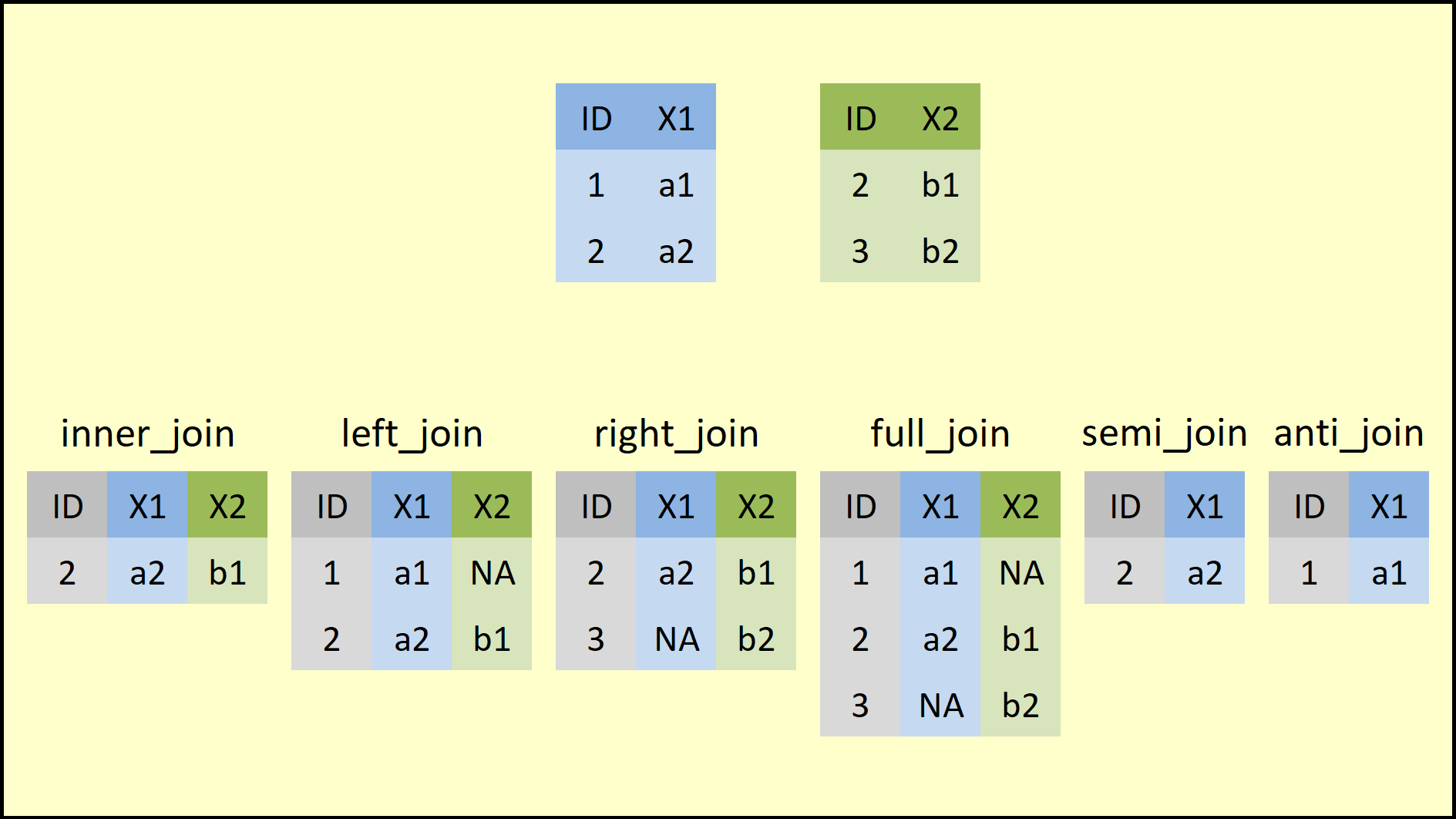
Figure 1.1: Overview of the dplyr Join Functions.

On the top of Figure 1, you can see the structure of the example data frames. Both data frames contain two columns: The ID and one variable (e.g, X1, X2). Note that both data frames have the ID=2 in common.

On the bottom row of Figure 1, you can see how each of the join functions merges two example data frames. Figure 1 summarizes the big picture of how the join function family works.

2 Load {dplyr} package

Before we can apply all the join functions, we need to install and load the {dplyr} package (I’ve already installed and loaded this package on my PC. So the load package step is just for demonstration purpose).

# load pacakge
library(dplyr)

3 Function 1: inner_join

inner_join produces only the set of records that match in both Table A and Table B. It is the most commonly used join function.

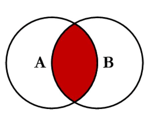
Figure 3.1: Inner Join

In this first example, I apply the inner_join function to our example data.

In order to merge our data based on inner_join, we simply have to specify the names of our two data frames (i.e. data1 and data2) and the column based on which we want to merge (i.e. the column ID):

# Apply inner_join dplyr function
inner_join(data1, data2, by = "ID")                

##   ID X1 X2
## 1  2 a2 b1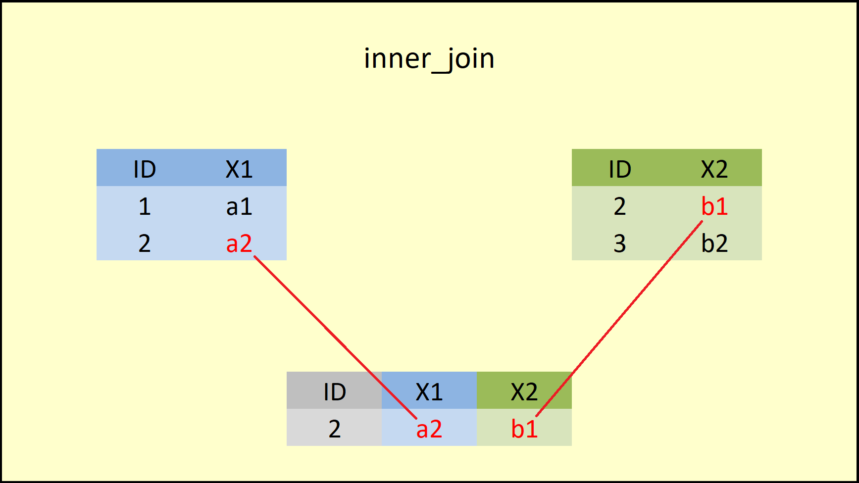

Figure 3.2: dplyr inner_join Function.

Figure 3.2 illustrates the output of the inner join that we have just performed. As you can see, the inner_join function merges the variables of both data frames, but retains only rows with a shared ID (i.e. ID=2).

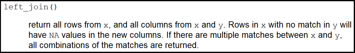
More precisely, this is what the R documentation is saying:

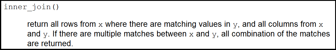
4 Function 2: left_join

The left_join function from {dplyr} package is similar to the left outer join function in SQL. It produces a complete set of records from Table A, with the matching records (where available) in Table B. If there is no match, the right side will contain null.

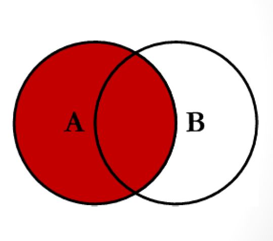
Figure 4.1: left_join

The left_join function can be applied as follows:

# Example 2: left_join dplyr R Function
left_join(data1, data2, by = "ID")                 

##   ID X1   X2
## 1  1 a1 <NA>
## 2  2 a2   b1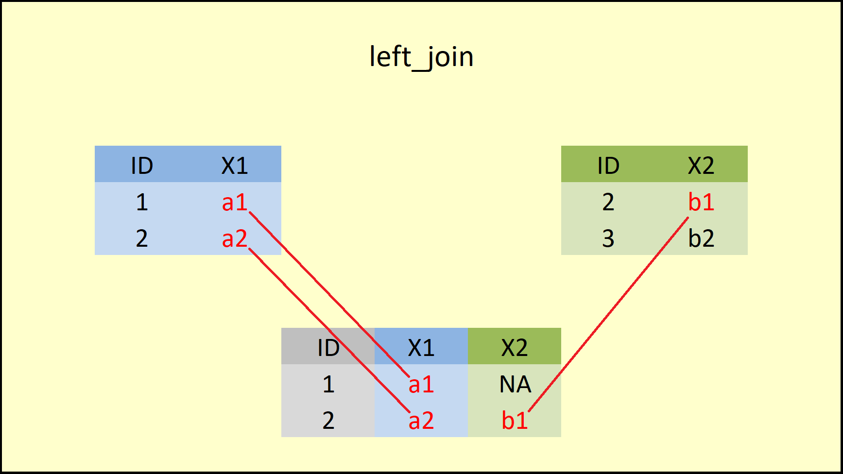

Figure 4.2: dplyr left_join Function.

The difference to the inner_join function is that left_join retains all rows of the data table, which is inserted first into the function (i.e. the X-data).

Have a look at the R documentation for a precise definition:

5 Function 3: right_join

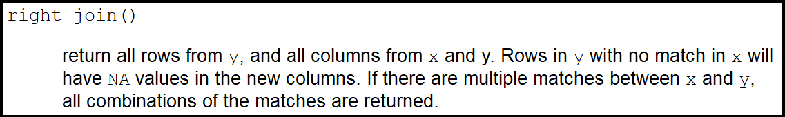
The right_join function from {dplyr} package is similar to the right outer join function in SQL. right_join produces a complete set of records from Table B, with the matching records (where available) in Table A. If there is no match, the left side will contain null.

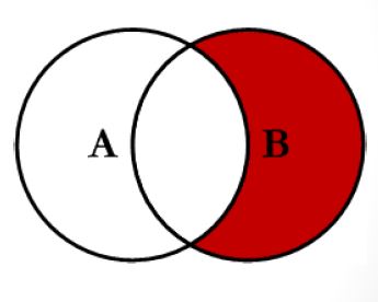
Figure 5.1: right join

As you can see from the Venn diagram, right join is the reversed function of left join:

# Example 3: right_join dplyr R Function
right_join(data1, data2, by = "ID")                # Apply right_join dplyr function

##   ID   X1 X2
## 1  2   a2 b1
## 2  3 <NA> b2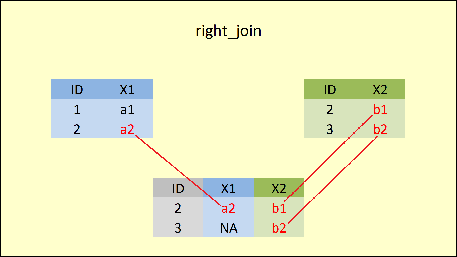

Figure 5.2: dplyr right_join Function.

Figure 5.2 shows that the right_join function retains all rows of the data on the right side (i.e. the Y-data). If you compare left join vs. right join, you can see that both functions are keeping the rows of the opposite data.

This behavior is also documented in the definition of right_join below:

So what if we want to keep all rows of our data tables?

6 Function 4: full_join

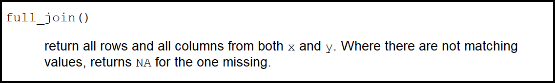
The full_join function from {dplyr} package is similar to the full outer join function in SQL. It produces the set of all records in Table A and Table B, with matching records from both sides where available. If there is no match, the missing side will contain null.

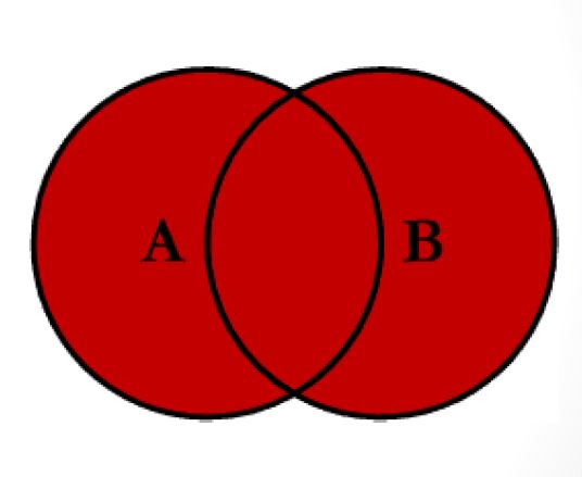
Figure 6.1: full join

A full_join retains the most data of all the join functions. Let’s have a look:

# Example 4: full_join dplyr R Function
full_join(data1, data2, by = "ID")                 

##   ID   X1   X2
## 1  1   a1 <NA>
## 2  2   a2   b1
## 3  3 <NA>   b2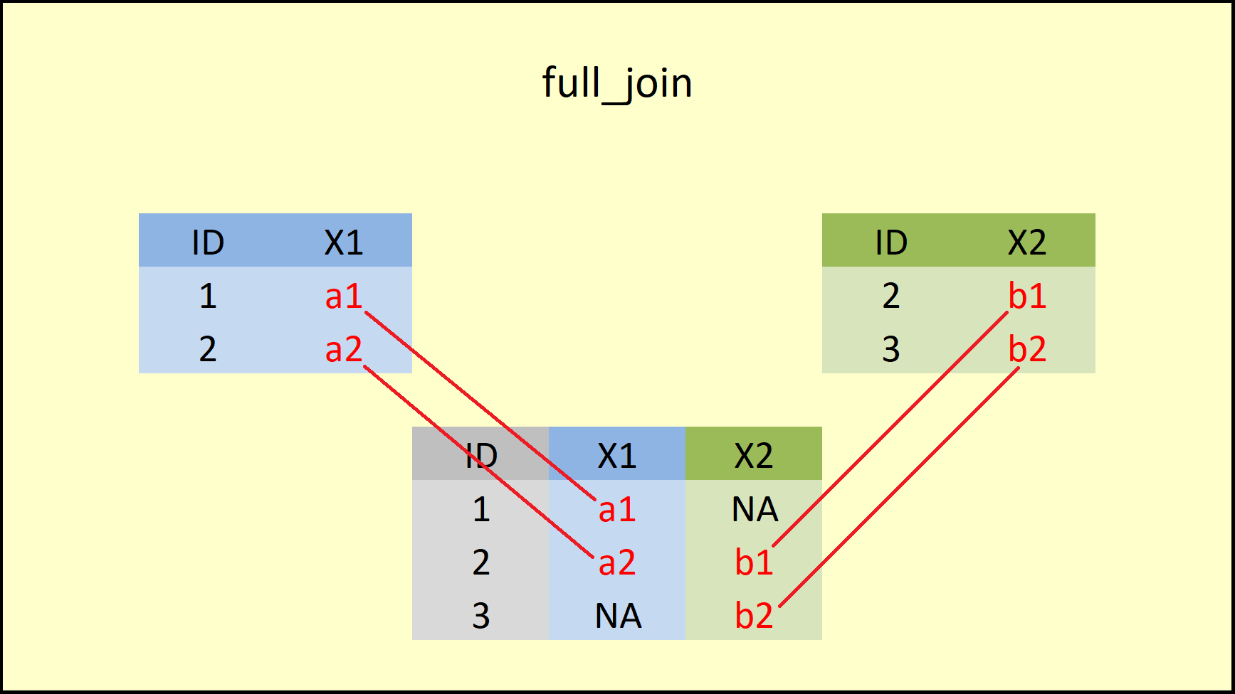

Figure 6.2: dplyr full_join Function.

As Figure 6.2 illustrates, the full_join functions retains all rows of both input data sets and inserts NA when an ID is missing in one of the data frames.

You can find the help documentation of full_join below:

7 Function 5: semi_join

The four previous join functions (i.e. inner_join, left_join, right_join, and full_join) are so called mutating joins. Mutating joins combine variables from the two data sources.

The next two join functions (i.e. semi_join and anti_join) are so called filtering joins. Filtering joins keep cases from the left data table (i.e. the X-data) and use the right data (i.e. the Y-data) as filter.

Let’s have a look at semi join first:

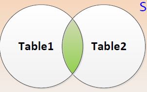
Figure 7.1: semi join

# Example 5: semi_join dplyr R Function (filtering joins)
# Only keep the variable from data1
semi_join(data1, data2, by = "ID")                 # Apply semi_join dplyr function

##   ID X1
## 1  2 a2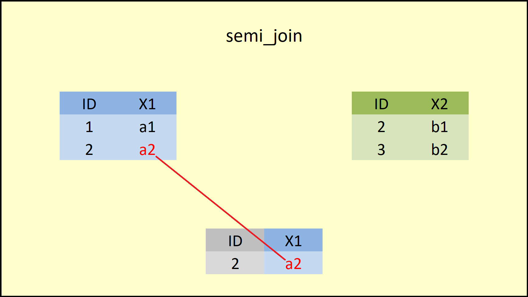

Figure 7.2: dplyr semi_join Function.

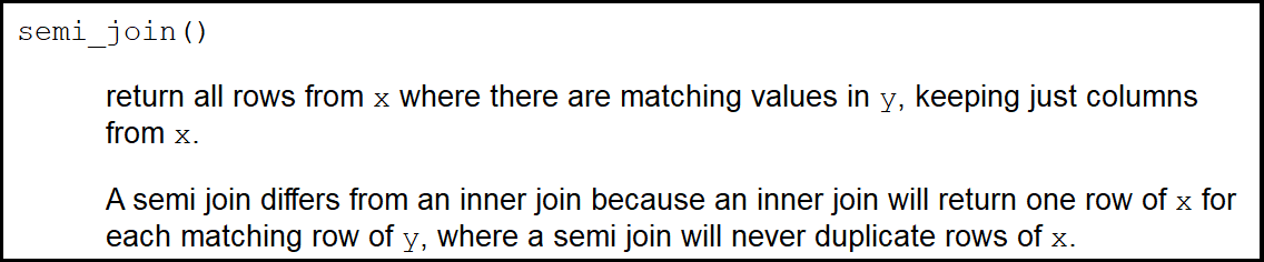
Figure 7.2 illustrates what is happening here: The semi_join function retains only rows that both data frames have in common AND only columns of the left-hand data frame. You can find a precise definition of semi join below:

8 Function 6: anti_join

anti_join does the opposite of semi_join:

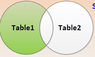
Figure 8.1: anti join

# Example 6: anti_join dplyr R Function (Only keep the variable from data1)
anti_join(data1, data2, by = "ID")                 # Apply anti_join dplyr function

##   ID X1
## 1  1 a1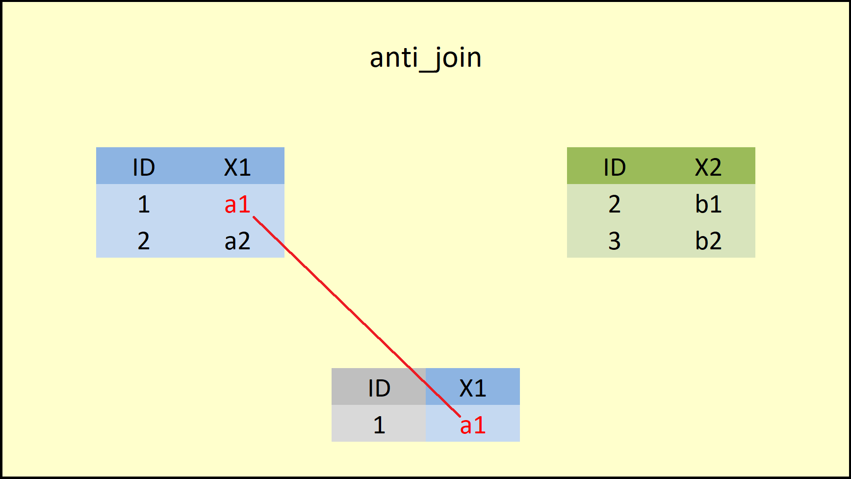

Figure 8.2: dplyr anti_join Function.

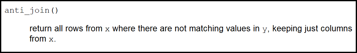
As you can see, the anti_join functions keeps only rows that are non-existent in the right-hand data AND keeps only columns of the left-hand data. The R help documentation of anti join is shown below:

At this point, you have seen the basic principles of the six dplyr join functions. However, in practice the data is of cause much more complex than in the previous examples.

In the remaining blog, I will apply the join functions in more complex data situations.

9 Complex Example 1: Join Multiple Data Frames

To make the remaining examples a bit more complex, I’m going to create a third data frame:

data3 <- data.frame(ID = c(2, 4),                   # Create third example data frame
                    X2 = c("c1", "c2"),
                    X3 = c("d1", "d2"),
                    stringsAsFactors = FALSE)
data3                                               # Print data to RStudio console

##   ID X2 X3
## 1  2 c1 d1
## 2  4 c2 d2

The third data frame data3 also contains an ID column as well as the variables X2 and X3. Note that the variable X2 also exists in data2.

In this example, I’ll explain how to merge multiple data sources into a single data set.

For the following examples, I am going to us the full_join function, but we could use every other join function the same way:

# how to merge multiple data sources 
full_join(data1, data2, by = "ID") %>%  # Full outer join of multiple data frames
  full_join(., data3, by = "ID") 

##   ID   X1 X2.x X2.y   X3
## 1  1   a1 <NA> <NA> <NA>
## 2  2   a2   b1   c1   d1
## 3  3 <NA>   b2 <NA> <NA>
## 4  4 <NA> <NA>   c2   d2

As you can see based on the previous code and the RStudio console output:

1. We first merged data1 and data2 and then,
2. in the second line of code, we added data3.

Note that X2 was duplicated, since it exists in data1 and data2 simultaneously. In the next example, I’ll show you how you might deal with that.

10 Complex example 2: Join by Multiple Columns

As you have seen in the previous example, data2 and data3 share several variables (i.e. ID and X2). If we want to combine two data frames based on multiple columns, we can select several joining variables for the by option simultaneously:

# Example 8: Join by Multiple Columns
full_join(data2, data3, by = c("ID", "X2"))         # Join by multiple columns

##   ID X2   X3
## 1  2 b1 <NA>
## 2  3 b2 <NA>
## 3  2 c1   d1
## 4  4 c2   d2

Note: The row of ID No. 2 was replicated, since the row with this ID contained different values in data2 and data3.

11 Complex example 3: Join Data & Delete ID

In the last example, I want to show you a simple trick, which can be helpful in practice. Often you won’t need the ID, based on which the data frames where joined, anymore. In order to get rid of the ID efficiently, you can simply use the following code:

# Example 9: Join Data & Delete ID
inner_join(data1, data2, by = "ID") %>%              # Automatically delete ID
  select(- ID)

##   X1 X2
## 1 a2 b1

That’s all I like to share. Thank you for reading.

I have also created a github repo, called-nine_join and uploaded all the useful materials for you to have a better understanding of the join function family.

You can download the example R script from this link: Code.

And some supplementary handouts are saved at Handout.

All the best~